Neural Network and Backpropagation (Chain Rule)

History and recent surge

From Wang and Raj (2017):

In a famous competition in 2012, the AlexNet (60 million weights) classified 1.2 million images in ImageNet with an error rate half of the next best one. This brings the current wave of deep learning.

Learning sources

• Linear Algebra and Learning from Data by Gil Strang.

• Elements of Statistical Learning (ESL) Chapter 11: https://web.stanford.edu/~hastie/ElemStatLearn/.

• UFLDL: http://ufldl.stanford.edu/tutorial/.

• Stanford CS231n: http://cs231n.github.io.

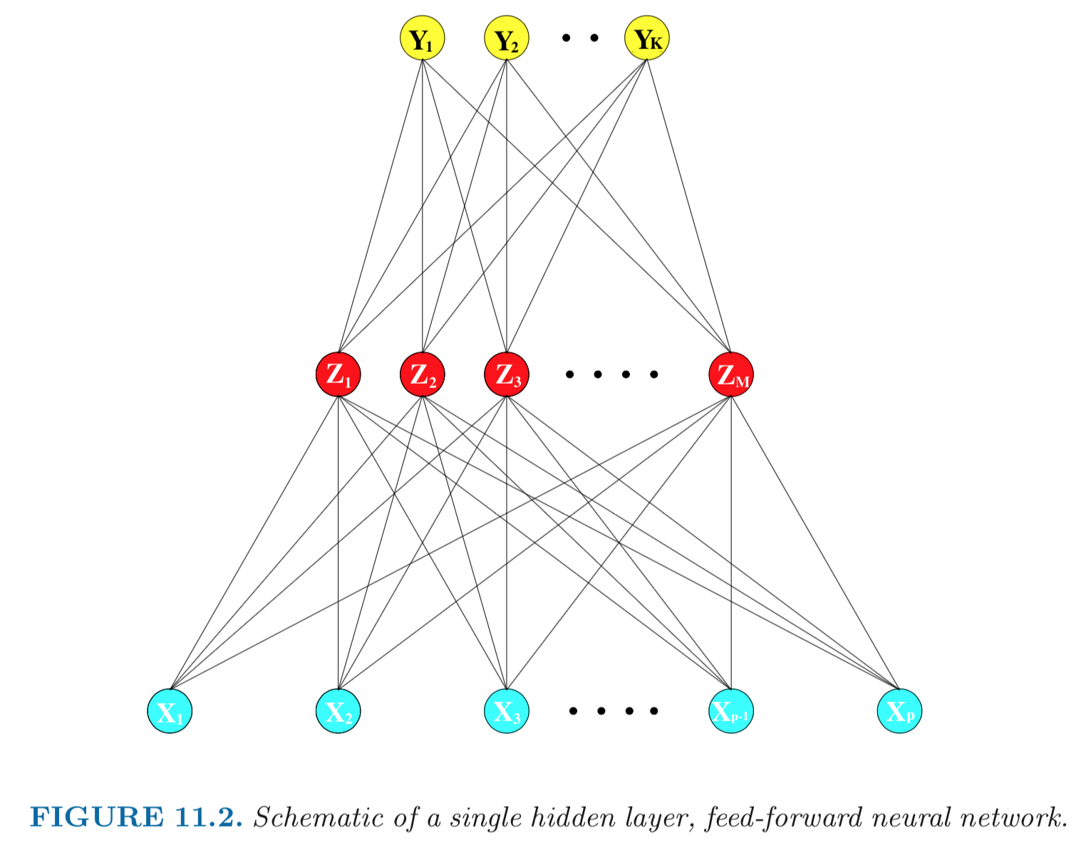
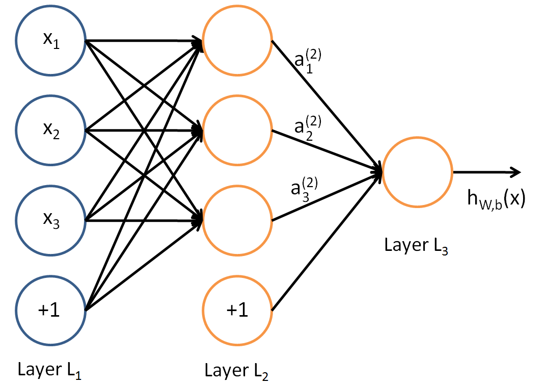
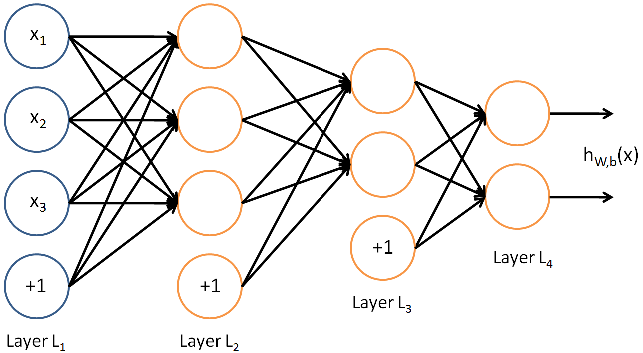
Single layer neural network (SLP)

• Aka single layer perceptron (SLP) or single hidden layer back-propagation network.

• Sum of nonlinear functions of linear combinations of the inputs, typically represented by a network diagram.
  

  TODO: redo above diagram to match notations.

• Mathematical model: $$ \mathbf{w} = \mathbf{A}_2[(\mathbf{A}_1 \mathbf{v}_0 + \mathbf{b}_0)_+]. $$

  • Input layer: $\mathbf{v}_0=(v_{01}, \ldots, v_{0p})$ are $p$-dimensional input features.

  • Hidden layer: $\mathbf{v}_1 = \mathbf{A}_1 \mathbf{v}_0 + \mathbf{b}_1$ are derived features created from linear combinations of inputs $\mathbf{v}$.

  • Activation function: A nonlinear activation function, e.g., $\text{ReLU}(x) = x_+ = \max(x, 0)$, is applied componentwise to the derived features to produce $(\mathbf{v}_1)_+ = (\mathbf{A}_1 \mathbf{v}_0 + \mathbf{b}_1)_+$.

  • Output layer: A function maps the derived features to the $K$-dimensional output. For example, $$ \mathbf{v}_1 \mapsto \mathbf{A}_2 \mathbf{v}_1 + \mathbf{b}_2, $$ where $\mathbf{A}_2 \in \mathbb{R}^{K \times q}$ and $\mathbf{b}_2 \in \mathbb{R}^K$.

  • Loss function: A loss function $L(\mathbf{w}, \mathbf{y})$ that measures the fitness of the output $\mathbf{w}$ to training labels.

  • Number of weights (parameters) is $q(p+1) + K(q+1)$.

• Activation function $\sigma$:

  • $\sigma(v)=$ a step function: human brain models where each unit represents a neuron, and the connections represent synapses; the neurons fired when the total signal passed to that unit exceeded a certain threshold.

  • Sigmoid function:
    $$ \sigma(v) = \frac{1}{1 + e^{-v}}. $$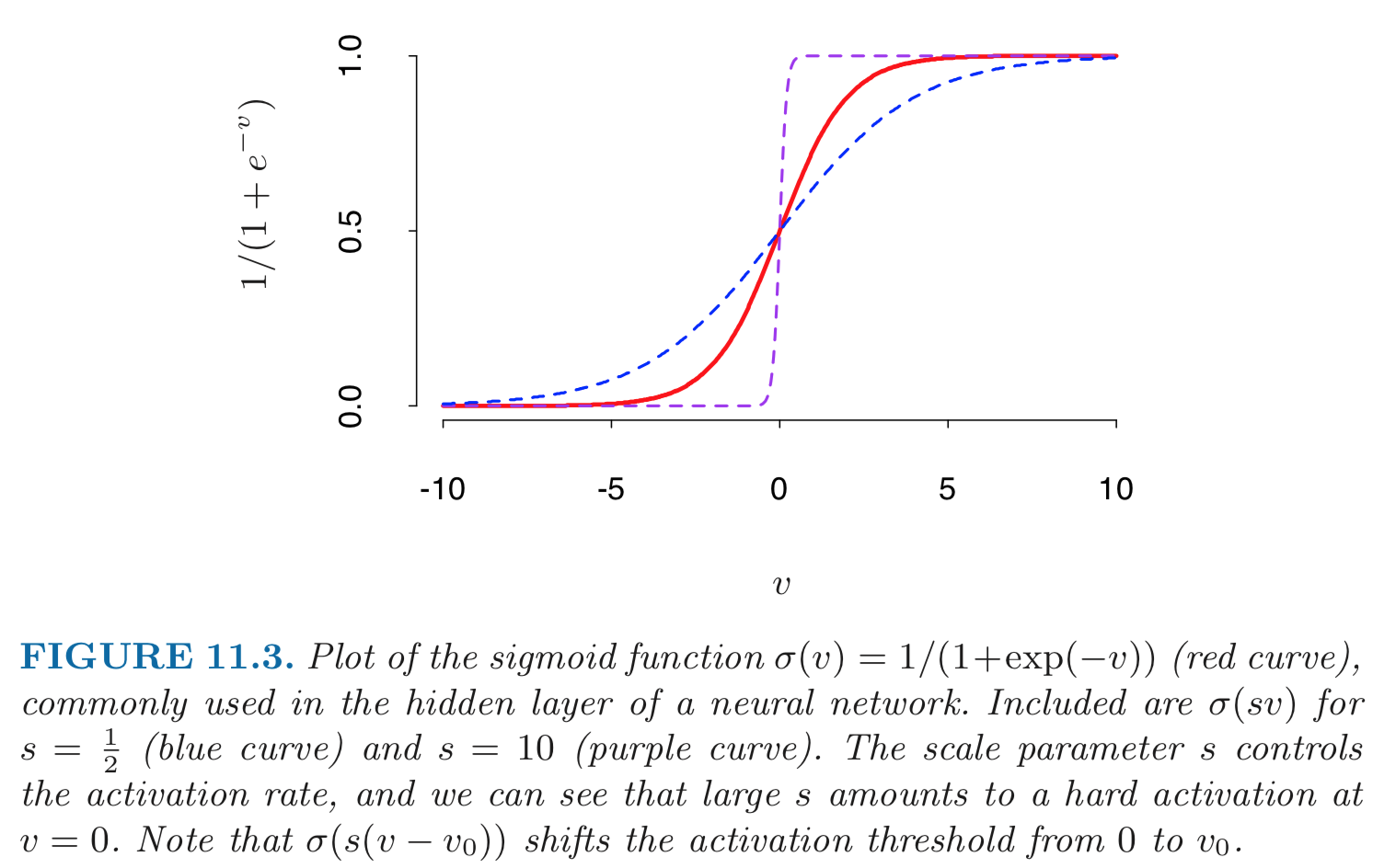

  • Rectifier. $\sigma(v) = v_+ = max(0, v)$. A unit employing the rectifier is called a rectified linear unit (ReLU). According to Wikipedia: The rectifier is, as of 2018, the most popular activation function for deep neural networks.

  • Softplus. $\sigma(v) = \log (1 + \exp v)$.
    

• Loss function: Given training data $(\mathbf{v}_{0,1}, y_1), \ldots, (\mathbf{v}_{0,n}, y_n)$, the loss function $L$ can be:

  • Sum of squared error (SSE): $$ L = \frac 12 \sum_{k=1}^K \sum_{i=1}^n [y_{ik} - w_{ik}]^2. $$

  • Cross-entropy (deviance): $$ L = - \sum_{k=1}^K \sum_{i=1}^n y_{ik} \log p_{ik}. $$ For $K$-class classification, $k$-th unit models the probability of class $k$. The softmax function $$ p_{ik} = \frac{e^{w_k}}{\sum_k e^{w_k}}, \quad k = 1,\ldots,K. $$

• Model fitting: back-propagation (gradient descent) to find the weights $\mathbf{A}_i, \mathbf{b}_i$ that minimize the loss function.

  • For notational simplicity, let's ignore the bias/intercept term $\mathbf{b}_1$.

  • Then the network structure is $$ \mathbf{v}_0 \mapsto \mathbf{v}_1 = \mathbf{A}_1 \mathbf{v}_0 \mapsto \mathbf{w} = \mathbf{A}_2 \sigma(\mathbf{v}_1) \mapsto L(\mathbf{w}, \mathbf{y}) $$ or $$ L(\mathbf{v}_0, \mathbf{y}) = L(\mathbf{A}_2\sigma(\mathbf{A}_1\mathbf{v}_0), \mathbf{y}). $$

  • Consider the sum of squared error with $K=1$ \begin{eqnarray*} L = \sum_i L_i, \text{ where } L_i &=& (y_i - w_i)^2. \end{eqnarray*}

  • The derivatives for the $i$-th training data point: \begin{eqnarray*} \frac{\partial L_i}{\partial \mathbf{A}_2} &=& \frac{\partial L_i}{\partial w_i} \cdot \frac{\partial w_i}{\partial \mathbf{A}_2} = - (y_{i} - w_i) \sigma(\mathbf{v}_{1,i}) \\ \frac{\partial L_i}{\partial \mathbf{A}_1} &=& \frac{\partial L_i}{\partial w_i} \cdot \frac{\partial w_i}{\partial \mathbf{v}_{1,i}} \cdot \frac{\partial \mathbf{v}_{1,i}}{\partial \mathbf{A}_1} = - (y_{i} - w_i) \text{diag}(\sigma'(\mathbf{v}_{1,i})) \mathbf{A}_2' \mathbf{v}_{0,i}'. \end{eqnarray*}
    Above is bad notation. Next lecture we learn how to derive chain rule properly.

  • Gradient descent update: \begin{eqnarray*} \mathbf{A}_{2}^{(t+1)} &=& \mathbf{A}_{2}^{(t)} - s^{(t)} \sum_{i=1}^n \frac{\partial L_i}{\partial \mathbf{A}_{2}^{(t)}} \\ \mathbf{A}_{1}^{(t+1)} &=& \mathbf{A}_{1}^{(t)} - s^{(t)} \sum_{i=1}^n \frac{\partial L_i}{\partial \mathbf{A}_{1}^{(t)}}, \end{eqnarray*} where $s^{(t)}$ is the learning rate.

  • Two-pass updates: for each training data point, \begin{eqnarray*} & & \text{current } \mathbf{A}_1, \mathbf{A}_2 \to \mathbf{v}_{1,i} \to \mathbf{w}_i \to \text{ evalulate loss } L_i \quad \quad \quad \text{(forward pass)} \\ &\to& \text{evaluate } \frac{\partial L_i}{\partial \mathbf{A}_2} \to \text{evaluate } \frac{\partial L_i}{\partial \mathbf{A}_1} \to \text{ update } \mathbf{A}_2 \text{ and } \mathbf{A}_1 \quad \quad \text{(backward pass)}. \end{eqnarray*}

  • Advantages: each hidden unit passes and receives information only to and from units that share a connection; can be implemented efficiently on a parallel architecture computer.

• Stochastic gradient descent (SGD). In real machine learning applications, training set can be large. Backpropagation over all training cases can be expensive. Learning can also be carried out online — processing each batch one at a time, updating the gradient after each training batch, and cycling through the training cases many times. A training epoch refers to one sweep through the entire training set.

  AdaGrad, RMSProp, and ADAM improve the stability of SGD by trying to incorpoate Hessian information in a computationally cheap way.

Expressivity of neural network

• Playground: http://playground.tensorflow.org

• Sources:

  • On the expressive power of deep neural network.
  • On the number of response regions of deep feed forward networks with piece-wise linear activations.

• Consider the function $F: \mathbb{R}^m \mapsto \mathbb{R}^n$ $$ F(\mathbf{v}) = \text{ReLU}(\mathbf{A} \mathbf{v} + \mathbf{b}). $$ Each equation $$ \mathbf{a}_i \mathbf{v} + b_i = 0 $$ creates a hyperplane in $\mathbb{R}^m$. ReLU creates a fold along that hyperplane. There are a total of $n$ folds.

  • When there are $n=2$ hyperplanes in $\mathbb{R}^2$, 2 folds create 4 pieces.
  • When there are $n=3$ hyperplanes in $\mathbb{R}^2$, 3 folds create 7 pieces.

• The number of linear pieces of $F$ and regions bounded by the $N$ hyperplanes is $$ r(n, m) = \sum_{i=0}^m \binom{n}{i} = \binom{n}{0} + \cdots + \binom{n}{m}. $$

  Proof: Induction using the recursion $$ r(n, m) = r(n-1, m) + r(n-1, m-1). $$

• Corollary:

  • When there are relatively few neurons $n \ll m$, $$ r(n,m) \approx 2^n. $$
  • When there are many neurons $n \gg m$, $$ r(n,m) \approx \frac{n^m}{m!}. $$

• Counting number of flat pieces with more hidden layers is much harder.

Multi-layer neural network (MLP) = function composition

• Aka multi-layer perceptron (MLP).

• 1 hidden layer:
  

• 2 hidden layers:
  

• In each layer, $$ \mathbf{v}_k = F_k(\mathbf{v}_{k-1}) = \text{ReLU}(\mathbf{A}_k \mathbf{v}_{k-1} + \mathbf{b}_k) $$ and the overall MLP with $L$ layers corresponds to function composition $$ \mathbf{w} = F_L(\ldots F_2(F_1(\mathbf{v}_0))). $$

Universal approximation properties

• Boolean Approximation: an MLP of one hidden layer can represent any boolean function exactly.

• Continuous Approximation: an MLP of one hidden layer can approximate any bounded continuous function with arbitrary accuracy.

• Arbitrary Approximation: an MLP of two hidden layers can approximate any function with arbitrary accuracy.

Practical issues

Neural networks are not a fully automatic tool, as they are sometimes advertised; as with all statistical models, subject matter knowledge should and often be used to improve their performance.

• Starting values: usually starting values for weights are chosen to be random values near zero; hence the model starts out nearly linear (for sigmoid), and becomes nonlinear as the weights increase.

• Overfitting (too many parameters):

  1. early stopping;
  2. weight decay by $L_2$ penalty
     $$ L(\mathbf{A}_1, \mathbf{A}_2) + \frac{\lambda}{2} \left( \|\mathbf{A}_1\|_{\text{F}}^2 + \|\mathbf{A}_2\|_{\text{F}}^2 \right), $$ where $\lambda$ is the weight decay parameter.
  3. Dropout. At each training case, individual nodes are either dropped out of the net with probability $1-p$ or kept with probability $p$, so that a reduced network is left; incoming and outgoing edges to a dropped-out node are also removed. Forward and backpropagation for that training case are done only on this thinned network.
     
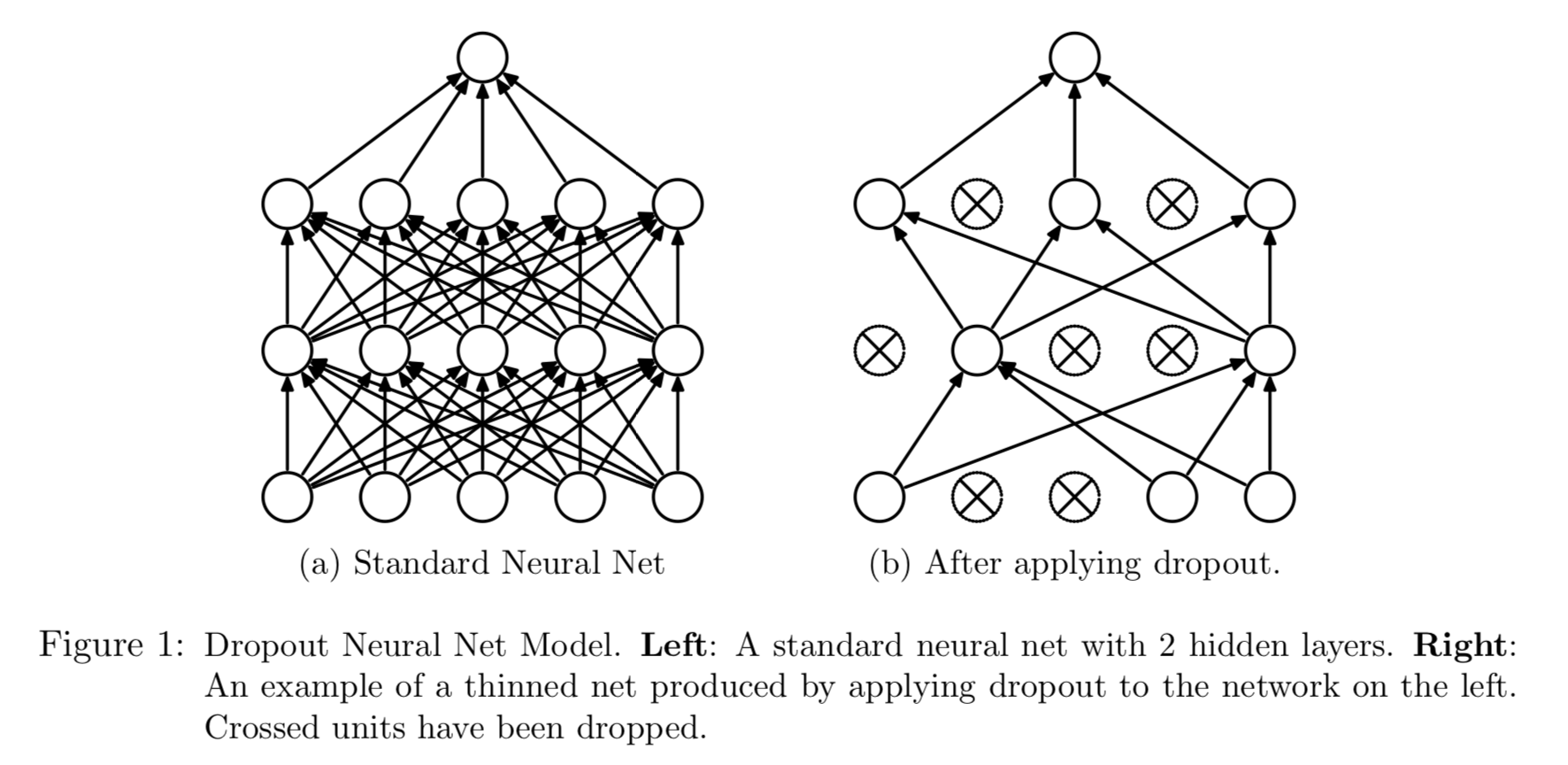
     Figure from Srivastava, Hinton, Krizhevsky, Sutskever, and Salakhutdinov (2014).

• Scaling of inputs: mean 0 and standard deviation 1. With standardized inputs, it is typical to take random uniform weights over the range [−0.7,+0.7].

• How many hidden units and how many hidden layers: guided by domain knowledge and experimentation.

• Multiple minima: try with different starting values.

Convolution neural network (CNN)

• CNN is a special structure in matrix $\mathbf{A}$ that utilizes the local stationarity of natural images.

• Stride, pooling, etc.

• Example: AlexNet for image classification.

• The structure of AlphaGo Zero:

  1. A convolution of 256 filters of kernel size $3 \times 3$ with stride 1.
  2. Batch normalization.
  3. ReLU.
  4. A convolution of 256 filters of kernel size $3 \times 3$ with stride 1.
  5. Batch normalization.
  6. A skip conneciton as in ResNets that adds the input to the block.
  7. ReLU.
  8. A fully connected linear layer to a hidden layer of size 256.
  9. ReLU.