Gram-Schmidt and QR Decomposition
In this lecture we (1) review the Gram-Schmidt (GS) algorithm to orthonormalize a set of vectors (or obtain an orthonormal basis of a column space), and (2) show that GS leads to the QR decomposition $\mathbf{A} = \mathbf{Q} \mathbf{R}$ of a rectangular matrix $\mathbf{A}$.

Example
Given $$ \mathbf{A} = \begin{pmatrix} 1 & 2 \\ 1 & 2 \\ 0 & 3 \end{pmatrix}, $$ how to find an orthonormal basis of $\mathcal{C}(\mathbf{A})$?
Step 1: Normalize $\mathbf{x}_1$: $$ \mathbf{q}_1 = \frac{\mathbf{x}_1}{\|\mathbf{x}_1\|} = \begin{pmatrix} \frac{1}{\sqrt 2} \\ \frac{1}{\sqrt 2} \\ 0 \end{pmatrix}. $$
Step 2: Project $\mathbf{x}_2$ to $\mathcal{C}(\{\mathbf{q}_1\})^\perp$ \begin{eqnarray*} & & (\mathbf{I} - \mathbf{P}_{\{\mathbf{q}_1\}}) \mathbf{x}_2 \\ &=& \mathbf{x}_2 - \mathbf{P}_{\{\mathbf{q}_1\}} \mathbf{x}_2 \\ &=& \mathbf{x}_2 - \langle \mathbf{q}_1, \mathbf{x}_2 \rangle \mathbf{q}_1 \\ &=& \begin{pmatrix} 2 \\ 2 \\ 3 \end{pmatrix} - 2 \sqrt 2 \begin{pmatrix} \frac{1}{\sqrt 2} \\ \frac{1}{\sqrt 2} \\ 0 \end{pmatrix} \\ &=& \begin{pmatrix} 0 \\ 0 \\ 3 \end{pmatrix}. \end{eqnarray*} and normalize $$ \mathbf{q}_2 = \frac{1}{3} \begin{pmatrix} 0 \\ 0 \\ 3 \end{pmatrix} = \begin{pmatrix} 0 \\ 0 \\ 1 \end{pmatrix}. $$
Therefore an orthonormal basis of $\mathcal{C}(\mathbf{A})$ is given by columns of $$ \mathbf{Q} = \begin{pmatrix} \frac{1}{\sqrt 2} & 0 \\ \frac{1}{\sqrt 2} & 0 \\ 0 & 1 \end{pmatrix}. $$ If we collect the inner products $\langle \mathbf{q}_i, \mathbf{x}_j \rangle$, $j \ge i$, into a matrix $\mathbf{R}$ $$ \mathbf{R} = \begin{pmatrix} \sqrt 2 & 2 \sqrt 2 \\ 0 & 3 \end{pmatrix}, $$ then we have $\mathbf{A} = \mathbf{Q} \mathbf{R}$.
Gram-Schmidt (GS) procedure and QR decomposition
Gram-Schmidt algorithm orthonormalizes a set of non-zero, linearly independent vectors $\mathbf{a}_1,\ldots,\mathbf{a}_n \in \mathbb{R}^m$.
- Initialize $\mathbf{q}_1 = \frac{\mathbf{a}_1}{\|\mathbf{a}_1\|_2}$
- For $k=2, \ldots, n$, $$ \begin{eqnarray*} \mathbf{v}_k &=& \mathbf{a}_k - \mathbf{P}_{{\cal C}\{\mathbf{q}_1,\ldots,\mathbf{q}_{k-1}\}} \mathbf{a}_k = \mathbf{a}_k - \sum_{j=1}^{k-1} \langle \mathbf{a}_k, \mathbf{q}_j \rangle \cdot \mathbf{q}_j \\ \mathbf{q}_k &=& \frac{\mathbf{v}_k}{\|\mathbf{v}_k\|_2} \end{eqnarray*} $$
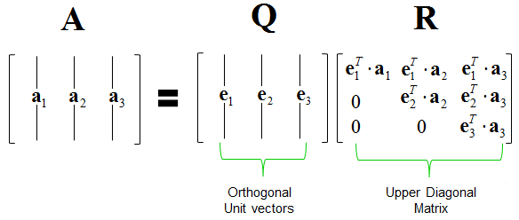
Collectively we have $\mathbf{A} = \mathbf{Q} \mathbf{R}$.
- $\mathbf{Q} \in \mathbb{R}^{m \times n}$ has orthonormal columns $\mathbf{q}_k$ thus $\mathbf{Q}^T \mathbf{Q} = \mathbf{I}_m$
- Where is $\mathbf{R}$? $\mathbf{R} = \mathbf{Q}^T \mathbf{X}$ has entries $r_{jk} = \langle \mathbf{q}_j, \mathbf{x}_k \rangle$, which are computed during the Gram-Schmidt process. Note $r_{jk} = 0$ for $j > k$, so $\mathbf{R}$ is upper triangular.
Computer actually performs QR on a column-permuted version of $\mathbf{A}$, that is $$ \mathbf{A} \mathbf{P} = \mathbf{Q} \mathbf{R}, $$ where $\mathbf{P}$ is a permutation matrix.
using LinearAlgebra

A = [1.0 2.0; 1.0 2.0; 0.0 3.0]
Aqr = qr(A)
Application to least squares problem
Recall that method of least squares minimizes $$ \|\mathbf{y} - \mathbf{X} \boldsymbol{\beta}\|^2 $$ to find the optimal vector in $\mathcal{C}(\mathbf{X})$ that approximates $\mathbf{y}$ best.
We showed that the least squares solution satisfies the normal equation $$ \mathbf{X}' \mathbf{X} \boldsymbol{\beta} = \mathbf{X}' \mathbf{y}. $$
If we are given the QR decomposition $\mathbf{X} = \mathbf{Q} \mathbf{R}$, then the normal equation becomes $$ \mathbf{R}' \mathbf{R} \boldsymbol{\beta} = \mathbf{X}' \mathbf{y}, $$ which is solved by two triangular solves.
This is how statistical software R solves the least squares or linear regression problem.