Linear equations and matrix inverses (BR Chapter 9)
Left and right inverses
A left inverse of $\mathbf{A} \in \mathbb{R}^{m \times n}$ is any matrix $\mathbf{B} \in \mathbb{R}^{n \times m}$ such that $\mathbf{B} \mathbf{A} = \mathbf{I}_n$.
A right inverse of $\mathbf{A} \in \mathbb{R}^{m \times n}$ is any matrix $\mathbf{C} \in \mathbb{R}^{n \times m}$ such that $\mathbf{A} \mathbf{C} = \mathbf{I}_m$.
BR Theorem 5.5. When does a matrix have a left or right inverse? Let $\mathbf{A} \in \mathbb{R}^{m \times n}$.
(1) $\mathbf{A}$ has a right inverse if and only if $\text{rank}(\mathbf{A}) = m$, or equivalently, $\mathbf{A}$ has full row rank.
(2) $\mathbf{A}$ has a left inverse if and only if $\text{rank}(\mathbf{A}) = n$, or equivalently, $\mathbf{A}$ has full column rank.Proof of (1). For the if part, since column rank equals row rank, the columns of $\mathbf{A}$ span $\mathbb{R}^m$. Then for each column $\mathbf{e}_j$ of $\mathbf{I}_m$, there exists $\mathbf{c}_j$ such that $\mathbf{A} \mathbf{c}_j = \mathbf{e}_j$. Collecting $\mathbf{c}_j$ as columns of $\mathbf{C}$, we proved $\mathbf{A} \mathbf{C} = \mathbf{I}$.
For the only if part, since $\mathbf{A} \mathbf{C} = \mathbf{I}_m$, we have $m \ge \text{rank}(\mathbf{A}) \ge \text{rank}(\mathbf{A} \mathbf{C}) = \text{rank}(\mathbf{I}_m) = m$. Thus $\text{rank}(\mathbf{A}) = m$.
Proof of (2). Apply (1) to $\mathbf{A}'$.
BR Theorem 5.6. If $\mathbf{A} \in \mathbb{R}^{m \times n}$ has a left inverse $\mathbf{B}$ and a right inverse $\mathbf{C}$. Then
(1) $\mathbf{A}$ must be a square, nonsingular matrix and $\mathbf{B} = \mathbf{C}$.
(2) $\mathbf{A}$ has a unique left inverse and a unique right inverse, which we call the inverse of $\mathbf{A}$ and denote it by $\mathbf{A}^{-1}$.Proof: From previous theorem, we have $m = \text{rank}(\mathbf{A}) = n$. Thus $\mathbf{A}$ is square, and $\mathbf{B}$ and $\mathbf{C}$ as well. Then $$ \mathbf{B} = \mathbf{B} \mathbf{I}_n = \mathbf{B} (\mathbf{A} \mathbf{C}) = (\mathbf{B} \mathbf{A}) \mathbf{C} = \mathbf{C}. $$ To show the uniqueness of left inverse, suppose $\mathbf{D}$ is another left inverse. Then $$ \mathbf{D} \mathbf{A} = \mathbf{I}_n = \mathbf{B} \mathbf{A}. $$ Multiplying both sides on the right by right inverse $\mathbf{C}$, we obtain $\mathbf{D} = \mathbf{B}$. Thus left inverse is unique. Uniqueness of right inverse is shown in a similar fashion.
BR Theorem 5.7. Let $\mathbf{A} \in \mathbb{R}^{m \times n}$. Then (1) $\mathbf{A}$ has full column rank if and only if $\mathbf{A}'\mathbf{A}$ is nonsingular. In this case, $(\mathbf{A}'\mathbf{A})^{-1} \mathbf{A}'$ is a left inverse of $\mathbf{A}$.
(2) $\mathbf{A}$ has full row rank if and only if $\mathbf{A}\mathbf{A}'$ is nonsingular. In this case, $\mathbf{A}'(\mathbf{A}'\mathbf{A})^{-1}$ is a right inverse of $\mathbf{A}$.Proof: easy.
Generalized inverse and Moore-Penrose inverse
BR Definition 9.3. Let $\mathbf{A} \in \mathbb{R}^{m \times n}$. A matrix $\mathbf{G} \in \mathbb{R}^{n \times m}$ is called the Moore-Penrose inverse or MP inverse of $\mathbf{A}$ if it satisifes following four conditions:
(1) $\mathbf{A} \mathbf{G} \mathbf{A} = \mathbf{A}$. $\quad \quad$ (generalized inverse, $g_1$ inverse, or inner pseudo-inverse)
(2) $\mathbf{G} \mathbf{A} \mathbf{G} = \mathbf{G}$. $\quad \quad$ (outer pseudo-inverse)
(3) $(\mathbf{A} \mathbf{G})' = \mathbf{A} \mathbf{G}$.
(4) $(\mathbf{G} \mathbf{A})' = \mathbf{G} \mathbf{A}$.
We shall denote the Moore-Penrose inverse of $\mathbf{A}$ by $\mathbf{A}^+$.Any matrix $\mathbf{G} \in \mathbb{R}^{n \times m}$ that satisfies (1) is called a generalized inverse, or $g_1$ inverse, or inner pseudo-inverse. Denoted by $\mathbf{A}^-$ or $\mathbf{A}^g$.
Any matrix $\mathbf{G} \in \mathbb{R}^{n \times m}$ that satisfies (1)+(2) is called a reflective generalized inverse, or $g_2$ inverse, or outer pseudo-inverse. Denoted by $\mathbf{A}^*$.
BR Theorem 9.18. The Moore-Penrose inverse of any matrix $\mathbf{A}$ exists and is unique.
Proof of uniqueness: Let $\mathbf{G}_1, \mathbf{G}_2 \in \mathbb{R}^{n \times m}$ be two matrices satisfying properties (1)-(4). Then
$$ \mathbf{A} \mathbf{G}_1 = (\mathbf{A} \mathbf{G}_1)' = \mathbf{G}_1' \mathbf{A}' = \mathbf{G}_1' (\mathbf{A} \mathbf{G}_2 \mathbf{A})' = \mathbf{G}_1' \mathbf{A}' \mathbf{G}_2' \mathbf{A}' = (\mathbf{A} \mathbf{G}_1)' (\mathbf{A} \mathbf{G}_2)' = \mathbf{A} \mathbf{G}_1 \mathbf{A} \mathbf{G}_2 = \mathbf{A} \mathbf{G}_2. $$ Similarly, $$ \mathbf{G}_1 \mathbf{A} = (\mathbf{G}_1 \mathbf{A})' = \mathbf{A}' \mathbf{G}_1' = (\mathbf{A} \mathbf{G}_2 \mathbf{A})' \mathbf{G}_1' = \mathbf{A}' \mathbf{G}_2' \mathbf{A}' \mathbf{G}_1' = (\mathbf{G}_2 \mathbf{A})' (\mathbf{G}_1 \mathbf{A})' = \mathbf{G}_2 \mathbf{A} \mathbf{G}_1 \mathbf{A} = \mathbf{G}_2 \mathbf{A}. $$ Hence, $$ \mathbf{G}_1 = \mathbf{G}_1 \mathbf{A} \mathbf{G}_1 = \mathbf{G}_1 \mathbf{A} \mathbf{G}_2 = \mathbf{G}_2 \mathbf{A} \mathbf{G}_2 = \mathbf{G}_2. $$Proof of existence: TODO later. We construct a matrix that satisfies (1)-(4) using the singular value decomposition (SVD) of $\mathbf{A}$.
Following are true:
- $(\mathbf{A}^-)'$ is a generalized inverse of $\mathbf{A}'$.
- $(\mathbf{A}')^+ = (\mathbf{A}^+)'$.
- For any nonzero $k$, $(1/k) \mathbf{A}^-$ is a generalized inverse of $k \mathbf{A}$.
$(k \mathbf{A})^+ = (1/k) \mathbf{A}^+$.
Proof: Check properties (1)-(4).
Multiplication by generalized inverse does not change rank.
- $\mathcal{C}(\mathbf{A}) = \mathcal{C}(\mathbf{A} \mathbf{A}^-)$ and $\mathcal{C}(\mathbf{A}') = \mathcal{C}((\mathbf{A}^- \mathbf{A})')$.
$\text{rank}(\mathbf{A}) = \text{rank}(\mathbf{A} \mathbf{A}^-) = \text{rank}(\mathbf{A}^- \mathbf{A})$.
Proof of 1: We already know $\mathcal{C}(\mathbf{A}) \supseteq \mathcal{C}(\mathbf{A} \mathbf{A}^-)$. Now since $\mathbf{A} = \mathbf{A} \mathbf{A}^- \mathbf{A}$, we also have $\mathcal{C}(\mathbf{A}) \subseteq \mathcal{C}(\mathbf{A} \mathbf{A}^-)$.
Proof of 2: By definition of rank.
Generalized inverse has equal or larger rank. $\text{rank}(\mathbf{A}^-) \ge \text{rank}(\mathbf{A})$.
Proof: $\text{rank}(\mathbf{A}) = \text{rank}(\mathbf{A}\mathbf{A}^- \mathbf{A}) \le \text{rank}(\mathbf{A}\mathbf{A}^-) \le \text{rank}(\mathbf{A}^-)$.
Linear equations
- Solving linear system $$ \mathbf{A} \mathbf{x} = \mathbf{b}, $$ where $\mathbf{A} \in \mathbb{R}^{m \times n}$ (coefficient matrix), $\mathbf{x} \in \mathbb{R}^n$ (solution vector), and $\mathbf{b} \in \mathbb{R}^m$ (right hand side) is a central theme in linear algebra.
We care about two fundamental questions: (1) when does the linear system has solution, and (2) how to characterize the solution set.
When is there a solution? The following statements are equivalent:
- The linear system $\mathbf{A} \mathbf{x} = \mathbf{b}$ has a solution (consistent).
- $\mathbf{b} \in \mathcal{C}(\mathbf{A})$.
- $\text{rank}((\mathbf{A} : \mathbf{b})) = \text{rank}(\mathbf{A})$.
$\mathbf{A} \mathbf{A}^- \mathbf{b} = \mathbf{b}$ for any generalized inverse $\mathbf{A}^-$.
The last equivalence gives some intuition why $\mathbf{A}^-$ is called an inverse.Proof: $1 \Rightarrow 2 \Rightarrow 3 \Rightarrow 1$ is easy. We show $1 \Rightarrow 4 \rightarrow 1$.
Proof of $1 \Rightarrow 4$: If $\tilde{\mathbf{x}}$ is a solution, then $$ \mathbf{b} = \mathbf{A} \tilde{\mathbf{x}} = \mathbf{A}\mathbf{A}^- \mathbf{A} \tilde{\mathbf{x}} = \mathbf{A}\mathbf{A}^- \mathbf{b}. $$
Proof of $4 \Rightarrow 1$: Apparently $\tilde{\mathbf{x}} = \mathbf{A}^- \mathbf{b}$ is a solution.
What are the solutions? Let's first consider the homogeneous system: $\mathbf{A} \mathbf{x} = \mathbf{0}$. Note homogeneous system is always consistent (why?)
Theorem: $\tilde{\mathbf{x}}$ is a solution of $\mathbf{A} \mathbf{x} = \mathbf{0}$ if and only if $$ \tilde{\mathbf{x}} = (\mathbf{I}_n - \mathbf{A}^- \mathbf{A}) \mathbf{q} $$ for some $\mathbf{q} \in \mathbb{R}^n$.
Rephrase of this theorem: $\mathcal{N}(\mathbf{A}) = \mathcal{C}(\mathbf{I}_n - \mathbf{A}^- \mathbf{A})$.Proof of "if" part: Regardless value of $\mathbf{q}$, we have $$ \mathbf{A} \tilde{\mathbf{x}} = \mathbf{A} (\mathbf{I}_n - \mathbf{A}^- \mathbf{A}) \mathbf{q} = (\mathbf{A} - \mathbf{A} \mathbf{A}^- \mathbf{A}) \mathbf{q} = \mathbf{O} \mathbf{q} = \mathbf{0}. $$
Proof of "only if" part: If $\tilde{\mathbf{x}}$ is a solution, then we have $$ \tilde{\mathbf{x}} = (\mathbf{I}_n - \mathbf{A}^- \mathbf{A}) \mathbf{q}, $$ where $\mathbf{q} = \tilde{\mathbf{x}}$.What are the solutions? Now we can study the inhomogeneous system: $\mathbf{A} \mathbf{x} = \mathbf{b}$.
Theorem: If $\mathbf{A} \mathbf{x} = \mathbf{b}$ is consistent, then $\tilde{\mathbf{x}}$ is a solution to $\mathbf{A} \mathbf{x} = \mathbf{b}$ if and only if $$ \tilde{\mathbf{x}} = \mathbf{A}^- \mathbf{b} + (\mathbf{I}_n - \mathbf{A}^- \mathbf{A}) \mathbf{q} $$ for some $\mathbf{q} \in \mathbb{R}^n$.
Interpretation: "a specific solution" + "a vector in $\mathcal{N}(\mathbf{A})$".Proof: \begin{eqnarray*} & & \mathbf{A} \mathbf{x} = \mathbf{b} \\ &\Leftrightarrow& \mathbf{A} \mathbf{x} = \mathbf{A} \mathbf{A}^- \mathbf{b} \\ &\Leftrightarrow& \mathbf{A} (\mathbf{x} - \mathbf{A}^- \mathbf{b}) = \mathbf{0} \\ &\Leftrightarrow& \mathbf{x} - \mathbf{A}^- \mathbf{b} \in \mathcal{N}(\mathbf{A}) \\ &\Leftrightarrow& \mathbf{x} - \mathbf{A}^- \mathbf{b} = (\mathbf{I}_n - \mathbf{A}^- \mathbf{A}) \mathbf{q} \text{ for some } \mathbf{q} \in \mathbb{R}^n \\ &\Leftrightarrow& \mathbf{x} = \mathbf{A}^- \mathbf{b} + (\mathbf{I}_n - \mathbf{A}^- \mathbf{A}) \mathbf{q} \text{ for some } \mathbf{q} \in \mathbb{R}^n. \end{eqnarray*}
$\mathbf{A} \mathbf{x} = \mathbf{b}$ is consistent for all $\mathbf{b}$ if and only if $\mathbf{A}$ has full row rank.
Proof of "if" part: If $\mathbf{A}$ has full row rank, then the column rank of $\mathbf{A}$ is $m$ and $\mathcal{C}(\mathbf{A}) = \mathbb{R}^m$. Thus for any $\mathbf{b} \in \mathbb{R}^m$, there exists a solution $\mathbf{x}$.
Proof of "only if" part: $\mathbf{A} \mathbf{A}^- \mathbf{b} = \mathbf{b}$ for all $\mathbf{b} \in \mathbb{R}^m$. Take $\mathbf{b} = \mathbf{e}_i$ for $i=1,\ldots,m$. We have $\mathbf{A} \mathbf{A}^- = \mathbf{I}_m$. Thus $$ m = \text{rank}(\mathbf{I}_m) = \text{rank}(\mathbf{A} \mathbf{A}^-) \le \text{rank}(\mathbf{A}) \le m. $$If $\mathbf{A} \mathbf{x} = \mathbf{b}$ is consistent, then its solution is unique if and only if $\mathbf{A}$ has full column rank.
Proof of "if" part: If there are two solutions $\mathbf{A} \mathbf{x}_1 = \mathbf{b}$ and $\mathbf{A} \mathbf{x}_2 = \mathbf{b}$, then $\mathbf{A} (\mathbf{x}_1 - \mathbf{x}_2) = \mathbf{0}$, i.e., $\mathbf{x}_1 - \mathbf{x}_2 \in \mathcal{N}(\mathbf{A})$. By the rank-nullity theorem, the $\mathcal{N}(\mathbf{A}) = \{\mathbf{0}\}$. Thus $\mathbf{x}_1 = \mathbf{x}_2$.
Proof of "only if" part: By characterization of soultion set, uniqueness of solution implies $\mathcal{N}(\mathcal{A}) = \{\mathbf{0}\}$. Then by the rank-nullity theorem, $\mathbf{A}$ has full column rank.If $\mathbf{A}$ has full row and column rank, then $\mathbf{A}$ is non-singular and the unique solution is $\mathbf{A}^{-1} \mathbf{b}$ for any $\mathbf{b}$.
Application: least squares
Least squares problem: $$ \text{minimize}_{\boldsymbol{\beta}} \quad f(\boldsymbol{\beta}) = \frac 12 \|\mathbf{y} - \mathbf{X} \boldsymbol{\beta}\|^2. $$ Find the linear combination of columns of $\mathbf{X} \in \mathbb{R}^{n \times p}$ that approximates $\mathbf{y} \in \mathbb{R}^n$ best, or equivalently, find the vector in $\mathcal{C}(\mathbf{X})$ that approximates $\mathbf{y}$ best.
Setting the gradient of objective to zero $$ \nabla f(\boldsymbol{\beta}) = - \mathbf{X}' (\mathbf{y} - \mathbf{X} \boldsymbol{\beta}) = \mathbf{0} $$ leads to the normal equation $$ (\mathbf{X}' \mathbf{X}) \boldsymbol{\beta} = \mathbf{X}' \mathbf{y}. $$
Is there a solution to the normal equation?
Claim: the normal equation is always consistent. Why?
Is the solution minimizer to the least squares criterion?
Claim: any solution $\hat{\mathbf{b}}$ to the normal equation minimizes the least squares criterion.
Optimization argument: Any stationary point (points with zero gradient) of a convex function is a global minimum. Now the least squares criterion is convex because the Hessian $\nabla^2 f(\boldsymbol{\beta}) = \mathbf{X}' \mathbf{X}$ is positive semidefinite. Therefore any solution to the normal equation is a stationary point and thus a global minimum.
Direct verifcation: Let $\tilde{\boldsymbol{\beta}}$ be a solution to the normal equation. For arbitrary $\boldsymbol{\beta} \in \mathbb{R}^p$, \begin{eqnarray*} & & f(\boldsymbol{\beta}) - f(\tilde{\boldsymbol{\beta}}) \\ &=& \frac 12 \|\mathbf{y} - \mathbf{X} \boldsymbol{\beta}\|^2 - \frac 12 \|\mathbf{y} - \mathbf{X} \tilde{\boldsymbol{\beta}}\|^2 \\ &=& \left( \frac 12 \mathbf{y}' \mathbf{y} - \mathbf{y}' \mathbf{X} \boldsymbol{\beta} + \frac 12 \boldsymbol{\beta}' \mathbf{X}' \mathbf{X} \boldsymbol{\beta} \right) - \left( \frac 12 \mathbf{y}' \mathbf{y} - \mathbf{y}' \mathbf{X} \tilde{\boldsymbol{\beta}} + \frac 12 \tilde{\boldsymbol{\beta}}' \mathbf{X}' \mathbf{X} \tilde{\boldsymbol{\beta}} \right) \\ &=& - \mathbf{y}' \mathbf{X} (\boldsymbol{\beta} - \tilde{\boldsymbol{\beta}}) + \frac 12 \boldsymbol{\beta}' \mathbf{X}' \mathbf{X} \boldsymbol{\beta} - \frac 12 \tilde{\boldsymbol{\beta}}' \mathbf{X}' \mathbf{X} \tilde{\boldsymbol{\beta}} \\ &=& - \tilde{\boldsymbol{\beta}}' \mathbf{X}' \mathbf{X} (\boldsymbol{\beta} - \tilde{\boldsymbol{\beta}}) + \frac 12 \boldsymbol{\beta}' \mathbf{X}' \mathbf{X} \boldsymbol{\beta} - \frac 12 \tilde{\boldsymbol{\beta}}' \mathbf{X}' \mathbf{X} \tilde{\boldsymbol{\beta}} \\ &=& \frac 12 \tilde{\boldsymbol{\beta}}' \mathbf{X}' \mathbf{X} \tilde{\boldsymbol{\beta}} - \tilde{\boldsymbol{\beta}}' \mathbf{X}' \mathbf{X} \boldsymbol{\beta} + \frac 12 \boldsymbol{\beta}' \mathbf{X}' \mathbf{X} \boldsymbol{\beta} \\ &=& \frac 12 (\tilde{\boldsymbol{\beta}} - \boldsymbol{\beta})' \mathbf{X}' \mathbf{X} (\tilde{\boldsymbol{\beta}} - \boldsymbol{\beta}) \\ &=& \frac 12 \|\mathbf{X} (\tilde{\boldsymbol{\beta}} - \boldsymbol{\beta})\|^2 \\ &\ge& 0. \end{eqnarray*} Therefore $\tilde{\boldsymbol{\beta}}$ must be a global minimum of the least squares criterion $f(\boldsymbol{\beta})$.
When is the solution to the normal equation unique?
The least squares solution is unique if and only if $\mathbf{X}' \mathbf{X}$ is non-singular if and only if $\mathbf{X}$ has full column rank.
In general, we can characterize the set of least squares solutions as $$ \tilde{\boldsymbol{\beta}}(\mathbf{q}) = (\mathbf{X}' \mathbf{X})^- \mathbf{X}' \mathbf{y} + [\mathbf{I}_p - (\mathbf{X}' \mathbf{X})^- (\mathbf{X}' \mathbf{X})] \mathbf{q}, $$ where $\mathbf{q} \in \mathbb{R}^q$ is arbitrary. A specific solution is $$ \tilde{\boldsymbol{\beta}} = (\mathbf{X}' \mathbf{X})^- \mathbf{X}' \mathbf{y} $$ with fitted values $$ \hat{\mathbf{y}} = \mathbf{X} \tilde{\boldsymbol{\beta}} = \mathbf{X} (\mathbf{X}' \mathbf{X})^- \mathbf{X}' \mathbf{y}. $$
$(\mathbf{X}' \mathbf{X})^- \mathbf{X}'$ is a generalized inverse of $\mathbf{X}$.
Proof: We need to show $\mathbf{X} (\mathbf{X}' \mathbf{X})^- \mathbf{X}' \mathbf{X} = \mathbf{X}$, or equivalently $\mathbf{X} (\mathbf{I}_p - (\mathbf{X}' \mathbf{X})^- \mathbf{X}' \mathbf{X}) = \mathbf{O}$. But earlier we showed $\mathcal{C}(\mathbf{I}_p - (\mathbf{X}' \mathbf{X})^- \mathbf{X}' \mathbf{X}) = \mathcal{N}(\mathbf{X}' \mathbf{X})$ and $\mathcal{N}(\mathbf{X}' \mathbf{X}) = \mathcal{N}(\mathbf{X})$.
Projection
$\mathbf{A} \mathbf{A}^-$ is a projector into the column space $\mathcal{C}(\mathbf{A})$ along $\mathcal{N}(\mathbf{A}) = \mathcal{C}(\mathbf{I} - \mathbf{A} \mathbf{A}^-)$.
Proof: $\mathbf{A} \mathbf{A}^-$ is idempotent because $\mathbf{A} \mathbf{A}^- \mathbf{A} \mathbf{A}^- = \mathbf{A} \mathbf{A}^-$. Thus it projects into $\mathcal{C}(\mathbf{A} \mathbf{A}^-)$, which we have shown to be equal to $\mathcal{C}(\mathbf{A})$.
$\mathbf{I}_n - \mathbf{A}^- \mathbf{A}$ is a projector into the null space $\mathcal{N}(\mathbf{A})$ along $\mathcal{C}(\mathbf{A})$.
An example of generalized inverses
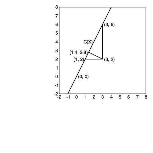
Let $$ \mathbf{A} = \begin{pmatrix} 1 \\ 2 \end{pmatrix} \in \mathbb{R}^{2 \times 1}. $$
What are generalized inverses of $\mathbf{A}$?
Let $$ \mathbf{A}^- = (u, v). $$ By definition of generalized inverse, we want $\mathbf{A} \mathbf{A}^- \mathbf{A} = \mathbf{A}$. That is \begin{eqnarray*} & & \begin{pmatrix} 1 \\ 2 \end{pmatrix} \begin{pmatrix} u, v \end{pmatrix} \begin{pmatrix} 1 \\ 2 \end{pmatrix} \\ &=& (u + 2v) \begin{pmatrix} 1 \\ 2 \end{pmatrix} \\ &=& \begin{pmatrix} u + 2v \\ 2u + 4v \end{pmatrix} \\ &=& \begin{pmatrix} 1 \\ 2 \end{pmatrix}, \end{eqnarray*} leading to the constraint $u + 2v = 1$, or, $v = (1-u)/2$. Thus any value of $u$ gives a generalized inverse $$ \mathbf{A}_u^- = \begin{pmatrix} u, \frac{1-u}{2} \end{pmatrix}. $$Visualize $\mathbf{A} \mathbf{A}^-$.
Take $u = 0$, then $$ \mathbf{A} \mathbf{A}_0^- = \begin{pmatrix} 1 \\ 2 \end{pmatrix} \begin{pmatrix} 0, \frac{1}{2} \end{pmatrix} = \begin{pmatrix} 0 & \frac 12 \\ 0 & 1 \end{pmatrix}. $$ Let's see how $\mathbf{A} \mathbf{A}_0^-$ acts on a vector $\mathbf{x} \in \mathbb{R}^2$: $$ \mathbf{A} \mathbf{A}_0^- \mathbf{x} = \begin{pmatrix} 0 & \frac 12 \\ 0 & 1 \end{pmatrix} \begin{pmatrix} x_1 \\ x_2 \end{pmatrix} = \begin{pmatrix} \frac{x_2}{2} \\ x_2 \end{pmatrix} = x_2 \begin{pmatrix} \frac 12 \\ 1 \end{pmatrix}. $$
Take $u = 1$, then $$ \mathbf{A} \mathbf{A}_1^- = \begin{pmatrix} 1 \\ 2 \end{pmatrix} \begin{pmatrix} 1, 0 \end{pmatrix} = \begin{pmatrix} 1 & 0 \\ 2 & 0 \end{pmatrix}. $$ Let's see how $\mathbf{A} \mathbf{A}_1^-$ acts on a vector $\mathbf{x} \in \mathbb{R}^2$: $$ \mathbf{A} \mathbf{A}_1^- \mathbf{x} = \begin{pmatrix} 1 & 0 \\ 2 & 0 \end{pmatrix} \begin{pmatrix} x_1 \\ x_2 \end{pmatrix} = \begin{pmatrix} x_1 \\ 2x_1 \end{pmatrix} = x_1 \begin{pmatrix} 1 \\ 2 \end{pmatrix}. $$
Take $u = \frac 15$ to make $\mathbf{A} \mathbf{A}_u^-$ symmetric: $$ \mathbf{A} \mathbf{A}_{1/5}^- = \begin{pmatrix} 1 \\ 2 \end{pmatrix} \begin{pmatrix} \frac 15, \frac 25 \end{pmatrix} = \begin{pmatrix} 1/5 & 2/5 \\ 2/5 & 4/5 \end{pmatrix}. $$ Let's see how $\mathbf{A} \mathbf{A}_{1/5}^-$ acts on a vector $\mathbf{x} \in \mathbb{R}^2$: $$ \mathbf{A} \mathbf{A}_{1/5}^- \mathbf{x} = \begin{pmatrix} 1/5 & 2/5 \\ 2/5 & 4/5 \end{pmatrix} \begin{pmatrix} x_1 \\ x_2 \end{pmatrix} = \begin{pmatrix} \frac{x_1 + 2x_2}{5} \\ \frac{2x_1 + 4x_2}{5} \end{pmatrix} = \frac{x_1 + 2x_2}{5} \begin{pmatrix} 1 \\ 2 \end{pmatrix}. $$